Experiments on communicating vessels, constrained optimization and manifolds
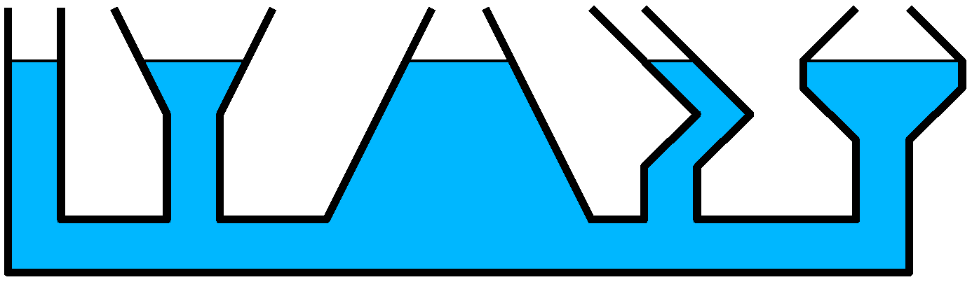
Image source 1.
Table of Contents
Fluid mechanics was one of my favourite topics in the Process Engineering program I followed (some people will quit reading at this point and never talk to me again) so without surprise, I could not resist diving into this new blog post on SIAM News. This is the second time a post from Mark Levi caught my attention, the last was on heat exchangers, on which I also wrote a post, toying with parallel and counter-current heat exchangers.
This new post from Mark Levi illustrates a key concept in constrained optimization: Lagrange multipliers and a nice interpretation in a problem of communicating vessels.
Communicating vessels and optimization formulation
If you are familiar with fluid mechanics, feel free to skip this section. Imagine $N$ vessels filled with water, all connected through a pipe at the bottom as shown on the top figure. The problem statement is, given initial levels of water $x_k$ in each $k-th$ vessel:
- how does the state evolve?
- what equilibrium, if any, is eventually reached?
Otherwise, consider the weight of water creates pressure within it. The lower a point in the water, the higher the pressure, since there is more water above which exercises its weight. A difference in pressure between two points will create a motion of the water, until the pressure equalizes. Put differently, some fluid moves from the full part of the vessel (with more pressure) to empty parts (with less pressure) until the pressure equalizes.
Since the pressure at a point depends on the height of the fluid above this point, two points have equal pressure when the height of water above them is equal. This is a phenomenon we often experience, with a watering can for instance.
Vessel equilibrium as an optimization problem
A system reaches an equilibrium at the minimum of its potential energy. Feel free to skip this part if you read the blog post by Mark Levi, we basically go over the problem formulation once again. An equilibrium state (where the state does not evolve anymore) can be found by solving the optimization problem minimizing the potential energy, subject to the respect of the laws of physics. These laws state two things:
- No water loss: the mass of liquid is preserved, and since we are working with an incompressible liquid, the total volume too is constant.
- No negative volume: the different vessels exchange water, their volume increasing or decreasing with time, but at no point can a vessel reach a negative volume.
Each vessel $k$ will be described by a profile, an area as function of the height $f_k(x)$. We assume that these functions $f_k$ are all continuous. The state at any point in time is the height in each vessel $x_k$. The total volume of water in the vessel is given by: $$V_k(x_k) = \int_0^{x_k} f_k(h) dh.$$
The conservation of volume can be expressed as:
$$V_{0} = \sum_{k=1}^N V_k(x_k) = \sum_{k=1}^N \int_0^{x_k} f_k(h) dh$$
where $V_{0}$ is the initial total volume water. The nonnegativity of water volume in each vessel can be expressed as: $$\int_0^{x_k} f_k(h) dh \geq 0,,, \forall k \in \{1..N\} $$
The area at any height $f_k(x)$ is positive or null, so this constraint can be simplified as: $$x_k \geq 0 ,,, \forall k \in \{1..N\} $$
The potential function, the objective minimized by the problem, is the last thing we miss. It consists of the total potential function of the water in the vessels, caused by gravity only. Each infinitesimal slice of water from $x$ to $x + dx$ exercises its weight, which is proportional to its volume $f_k(x) dx$ times height $x$. By integrating over a whole vessel $k$, this gives a potential of: $$ \int_0^{x_k} h f_k(h) M dh$$ with M a constant of appropriate dimension. Since we are minimizing the sum of these functions, we will get rid of the constant (sorry for shocking physicists), yielding an objective:
$$ F(x) = \sum_{k=1}^N \int_0^{x_k} h f_k(h)dh.$$
To sum it all, the optimization problem finding an equilibrium is:
$$
\begin{align}
\min_{x} & \sum_{k=1}^N \int_0^{x_k} h f_k(h)dh \\\\
& \text{subject to:} \\\
& G(x) = \sum_{k=1}^N \int_0^{x_k} f_k(h) dh - V_0 = 0\\\\
& x_k \geq 0 ,,, \forall k \in \{1..N\}
\end{align}
$$
If you read the blog post, you saw the best way to solve this problem is by relaxing the positivity constraints and write the first-order Karush-Kuhn-Tucker (KKT) conditions:
$$ \begin{align} & \nabla F(x) = \lambda \nabla G(x) & \Leftrightarrow\\\ & x_k f_k(x_k) = \lambda f_k(x_k) ,,,\forall k \in \{1..N\} & \Leftrightarrow \\\ & x_k = \lambda ,,,\forall k \in \{1..N\} \end{align} $$
So the multiplier $\lambda$ ends up being the height of water across all vessels, the equations come back to the intuitive result. Between the second and third line, we implicitly eliminate the case $f_k(x_k) = 0$, which would be a section of the vessel of area 0. Let us implement $F$, $G$ and their gradients in Julia to reproduce this result numerically. We will use four vessels of various shapes:
import QuadGK

const funcs = (
    x -> oneunit(x),
    x -> 2x,
    x -> 2 * sqrt(x),
    x -> 2 * x^2
)

const N = length(funcs)

g(x) = sum(1:N) do k
    QuadGK.quadgk(funcs[k], 0, x[k])[1]
end

f(x) = sum(1:N) do k
    x[k] * QuadGK.quadgk(funcs[k], 0, x[k])[1]
end
QuadGK.quadgk from the Gauss–Kronrod package
computes a numerical integral of a function on an interval.
We are in an interesting case where the gradient of the functions are much easier to
compute than the functions themselves, since they remove the integrals:
∇f(x) = [x[k] * funcs[k](x[k]) for k in 1:N]

∇g(x) = [funcs[k](x[k]) for k in 1:N]
If we pick a starting point, such that all four vessels have the same height:
x0_height = rand()
x0_uniform = [x0_height for _ in 1:N]
we can verify the first-order KKT conditions as expressed in Mark Levi’s post:
∇f(x0_uniform) - x0_height * ∇g(x0_uniform)
and we obtain a vector of zeros as planned.
The rest of this post will be about trying to find the optimal height that is reached by this system, implementing an iterative algorithm solving the problem in a generic form. This will require several parts:
- From a given iterate, find a direction to follow;
- Ensure each iterate respects the constraints defined above (no thugs in physicstown);
- Converge to the feasible solution (which we know from Mark Levi’s post, but no cheating);
- Define stopping criteria.
An interesting point on the structure of the problem, this is not a generic equality-constrained non-linear problem, the domain defined by $G(x) = 0$ is a manifold, which is a smooth subspace of $\mathbb{R}^N$. Other than throwing fancy words, having this structure lets us use specific optimization methods which have been developed for manifolds. A whole ecosystem has been developed in Julia to model and solve optimization problems over manifolds. We will not be using it and will build our method from scratch, inefficient but preferred for unknown reasons, like your sourdough starter in lockdown.
Computing a direction
From a given solution, we need to be able to find a direction in which we can progress. Fair warning, this is the most “optimization-heavy” section.
Let us start from a random point. Use the same seed if you want to reproduce the results:
Random.seed!(42)

# 4 uniform random points between [0,2]
x0 = 2 * rand(4)
V0 = g(x0)
# 1.9273890036845946
With the vessel shape functions defined above, this looks roughly like this:
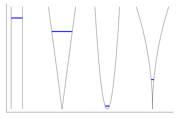
(source code available in the bonus section).
In unconstrained optimization, the gradient provides us with information on the steepest ascent direction, by following the opposite direction, the function will decrease, at least locally.
xnew = x_i - γ * ∇f(xinit)
See this good blog post by Ju Yang several with really good illustrations to grasp an intuition. If we naively follow the descent direction minimizing $F$, we likely leave the manifold, the region where $G(x) = 0$.
Think of the curve as the feasible region where we are supposed remain. $x_i$ is our current iterate and the direction points to the steepest descent of $F(x)$, i.e. $-\nabla F(x)$.
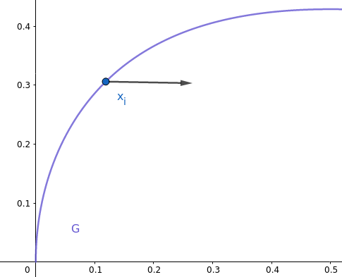
Moving in this direction will drive our iterates away from the feasible region, which is not desired. Instead, we will want to project this direction to follow the equality constraints, like the red direction:
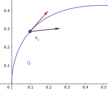
Of course, by following a fixed direction, the iterate ends up not on the curve, but not “too far”. More importantly, we will have ensured that the point has not been moved for nothing, which would be the case if we simply get away from the manifold. We are looking for a search direction $d$:
- which improves the objective function as much as possible: $\langle ∇F(x_{i}), d\rangle$ as low as possible, or equivalently $\langle -∇F(x_i), d\rangle$ maximized;
- tangent to the manifold.
For the last requirement, we need a direction in the tangent space to the manifold, so $\langle \nabla G(x_i), d\rangle = 0$, we end up requiring the vector rejection (the residual of a vector projection):
$$ \begin{align} & d = -\nabla F(x_i) - \frac{-\nabla F(x_i) \cdot \nabla G(x_i)}{\|\nabla G(x_i)\|^2} \nabla G(x_i) \Leftrightarrow \\\ & d = \frac{\nabla F(x_i) \cdot \nabla G(x_i)}{\|\nabla G(x_i)\|^2} \nabla G(x_i) -\nabla F(x_i) \end{align} $$
function compute_direction(grad_f, grad_g)
    return -grad_f + grad_g * (grad_f ⋅ grad_g) / (grad_g ⋅ grad_g)
end
Note: in a first version of this post, the projection was implemented as a Second-Order Cone problem (SOCP) in JuMP, which is computationally more expensive, just the first thing I thought of. When you are used to hammers, all projections look like nails. For curiosity, you will find it below:
$$ \begin{align} \min_{d, t} & \langle\nabla F(x_i), d \rangle \\\ & \text{subject to:} \\\ & \langle \nabla G(x_i), d\rangle = 0 \\\ & t = 1 \\\ & \|d\| \leq t \end{align} $$
The second-order cone constraint is $\|d\| \leq t$. Note that the direction is restricted to have unit $l_2$-norm, unlike the vector rejection above.
using JuMP
import ECOS

function compute_direction_SOCP(grad_f, grad_g)
    N = length(grad_f)
    m = Model(ECOS.Optimizer)
    MOI.set(m, MOI.Silent(), true)
    @variable(m, d[1:N])
    @constraint(m, grad_g ⋅ d == 0)
    @variable(m, t == 1)
    @constraint(m, [t;d] in SecondOrderCone())
    @objective(m, Min, d ⋅ grad_f)
    optimize!(m)
    termination_status(m) == MOI.OPTIMAL || error("Something wrong?")
    return JuMP.value.(d)
end
Also in the first version of this post, I had set the norm of $d$ to be equal to that of $\nabla F(x_i)$, which is a bad idea$^{TM}$. You will find in the bonus section the resulting descent.
On the point x0 defined above, the naive descent direction yields:
∇f(x0)
# 4-element Array{Float64,1}:
#  1.0663660320877226
#  1.649139647696062
#  0.013306072041938516
#  0.08274729914625051
and the projected gradient:
d = compute_direction(∇f(x0), ∇g(x0))
# 4-element Array{Float64,1}:
#  -0.7980557152422237
#  0.0054117074806136894
#  1.66214850442488
#  0.6812946467870831
Note that all elements in $∇f(x0)$ are positive, which makes sense from the intuition of the physics, the water in each vessel has a weight, thus exercising a pressure downwards.
There is still one thing we forgot once the direction is found.
Remember the positivity constraint $x_k \geq 0$?
It ensures the solution found makes sense, and that fluid mechanics
specialists won’t laugh at the solutions computed.
If one of the coordinates of the found point is negative,
what we can do is maintain the direction, but reduce the step.
Notice that one of our containers has an area of $2\sqrt{x}$,
reaching $x=0$ could lead to odd behaviour,
we will maintain the constraint x_k <= minval with
minval a small positive number.
function corrected_step(x, d, γ = 0.05; minval = 0.005)
    res = x + γ * d
    for k in eachindex(res)
        if res[k] < minval
            γ = (minval - x[k]) / d[k]
            res = x + γ * d
        end
    end
    return res
end
Note: in a general setting, a more appropriate method like the active set method
would have handled inequality constraints in a cleaner way.
In our case, if a height is close to 0, it will not stay there but
“bounce back”, so keeping track of active sets is unnecessary.
So we now have an iterate, the res variable returned from corrected_step,
which will always respect the positivity constraints and be improving the
objective in general.
Projecting on the manifold
We know in which direction $d$ the next iterate must be searched and have found an adequate step size $\gamma$, but a straight line can never perfectly stick to a curved surface. So once the direction is found and a new iterate $x_i + \gamma d$ computed, we need to project this iterate on the manifold, i.e. find the solution to:
$$ \begin{align} \min_{x}\,\, & dist(x, x_i + \gamma d) \\\ & \text{subject to:} \\\ & G(x) = 0 \end{align} $$
Sadly, this is where we need evaluations of $G(x)$, which is notably more expensive than its gradient. Evaluating $G(x_i + \gamma d)$ gives us either 0 (the volume conservation holds), a positive or negative quantity (for a volume creation or destruction). We can shift all the vessel heights by a same scalar $\alpha$ until $G(x_i + \gamma d + \alpha) = 0$.
function h(x)
    function(α)
        g(x .+ α) - V0
    end
end
h(corrected_step(x0, d, 1.5))(-0.5)
# -1.4234221843048611
h(corrected_step(x0, d, 1.5))(0.5)
# 3.5464645750853023
The problem then becomes a root-finding problem on $h(x)(\alpha)$. Typical methods for solving a root-finding problem are Newton-type methods, bisections. We will use the Roots.jl package, this post is already too long to implement one from scratch.
# computes the good alpha, starting from 0

root = Roots.find_zero(h(corrected_step(x0, d, 1.5)), 0.0)
# -0.07526921814981354

g(corrected_step(x0, d, 1.5) .+ root) - V0
# 0.0
Putting it all together
We now have all the ingredients to make this algorithm work:
Compute a gradient, correct it for negative points, project it on the manifold (with the simple vector rejection or the SOCP), re-project the resulting point with root-finding on alpha. We will stop the algorithm either:
- If a number of iterations is reached (which is considered a failure since we did not converge);
- The norm of the projected gradient is almost zero and we would not move to a new iterate;
- The distance between two successive iterates is low enough.
function find_equilibrium(funcs, x0; mingradnorm=10e-5, maxiter = 1000, γ = 0.05, mindiff=10e-4)
    xs = [x0]
    niter = 0
    while niter <= maxiter
        x = xs[end] # last iterate
        # compute projected direction
        d = compute_direction(∇f(x), ∇g(x))
        # keep new point in positive orthant
        xpos = corrected_step(x, d, γ)
        # project point on Manifold
        α = Roots.find_zero(h(xpos), 0.0)
        xnew = xpos .+ α
        push!(xs, xnew)
        niter += 1
        if norm(d) < mingradnorm
            @info "Min gradient condition reached"
            return xs
        end
        if norm(x - xnew) < mindiff
            @info "Min difference condition reached"
            return xs
        end
    end
    @info "Max iterations reached without convergence"
    return xs
end
Giving it a try with a first rough idea of parameters:
xs = find_equilibrium(funcs, x0, γ = 0.005, maxiter = 5000, mindiff=10e-6)
# Info: Min difference condition reached
We converged because the successive iterates were close enough, let us check the solution profile:
xs_pivot = map(1:4) do k
    getindex.(xs, k)
end

plot(xs_pivot)
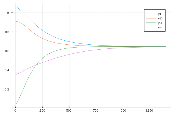
Fair enough, still, 1400 iterates should not be necessary for a 4-dimensional problem. Since convergence seems reached around the equilibrium point (the solution does not bounce around it), we can increase the step size, which was taken rather conservatively:
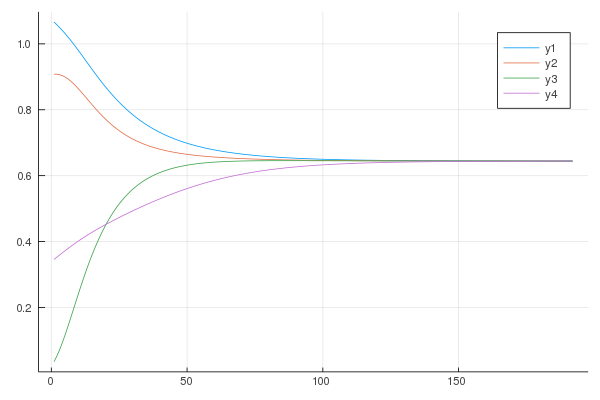
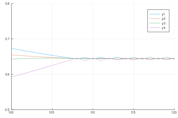
Let us zoom in:
xs = find_equilibrium(funcs, x0, γ = 0.05, maxiter = 5000, mindiff=10e-6)
plot(map(k -> getindex.(xs, k), 1:4))
We reduce the number of iterations to 192, while not hindering convergence.
Conclusion and perspective
I wanted to add a section on the corresponding dynamical system, namely a differential algebraic equation (DAE) system, but this is clearly long enough, and I couldn’t get anything to work.
TL;DR: the techniques to find the equilibrium rely on local optimization tools. The problem structure allowed us to express the gradient and estimate projection steps using cheap enough methods, namely vector rejection and root finding on a univariate function.
Interesting thing to do on top of this:
- Leverage the toolbox already present and coming in JuliaManifolds;
- Replace the gradient-based method used here with a higher-order one such as quasi-Newton, L-BFGS, which should come cheaply from the decomposability of both $F$ and $G$.
For the first point in particular, the direction projection can be seen as a retraction on the manifold. Thanks Ronny Bergmann for pointing it out!
A fixed step size worked out well in our case because the problem structure is smooth enough,
a better way would be doing a line search in the direction of $d$.
The LineSearches.jl package is readily available,
one could directly plug one of the available methods in the corrected_step function.
Finally, going back to the initial motivation of Mark Levi in the SIAM post, one can express the KKT conditions on a Manifold-constrained problem as developed in this article.
Acknowledgment
Special thanks to Pierre for reading this post and spotting errors quicker than I could type them, Antoine Levitt for highlighting the SOCP approach was awfully overkill for a gradient projection, this also made me spot an other error, and Ronny Bergmann for encouraging words and detailed feedback and discussion on different parts of the talk, from links with JuliaManifolds to incorrect terminology and improvement perspective. Thanks also to Chris for the conversation on DAEs, for another post maybe, Odelin for the suggestion on the variable notations. And as often, thanks Pierre-Yves for the infaillible proof-reading as usual.
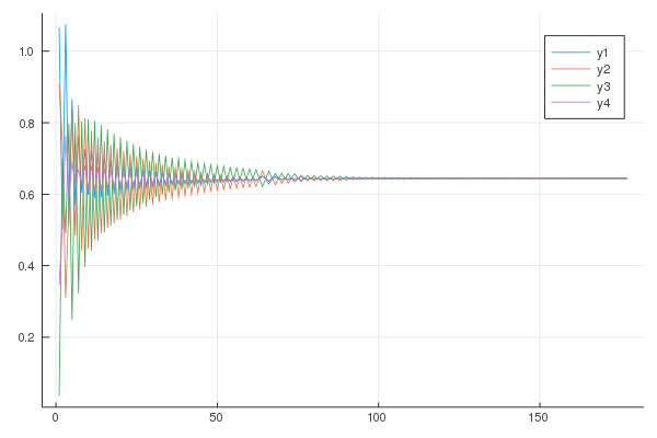
Bonus
What happens when the norm of the direction vector is proportional to $\nabla F(x_i)$ instead of the projected vector (or constant)? Don’t reproduce at home:
As promised, the plot to represent the vessels with the initial level of filling:
p = plot(xaxis=nothing, yaxis=nothing)
xtop = 1.2
xks = collect(0.0:0.01:xtop)
center_points = (-4N:4N)
for k in 1:N
    center_point = center_points[4k]
    rhs = [funcs[k](xki)/2 + center_point  for xki in xks]
    lhs = [-funcs[k](xki)/2 + center_point  for xki in xks]
    plot!(p, rhs, xks, color = "black", label = "")
    plot!(p, lhs, xks, color = "black", label = "")
    plot!(
        p,
        [-funcs[k](x0[k])/2 + center_point, funcs[k](x0[k])/2 + center_point],
        [x0[k], x0[k]],
        label = "",
        color = "blue",
        width = 3,
    )
end
The result is the plot presented in the introduction. A nice way to observe the evolution of the system is with this format directly:
function plot_containers(x, xaxis=nothing, yaxis=nothing, iter = 100)
    xtop = 1.2
    xks = collect(0.0:0.01:xtop)
    center_points = (-4N:4N)
    for k in 1:N
        center_point = center_points[4k]
        rhs = [funcs[k](xki)/2 + center_point  for xki in xks]
        lhs = [-funcs[k](xki)/2 + center_point  for xki in xks]
        plot!(p, rhs, xks, color = "black", label = "")
        plot!(p, lhs, xks, color = "black", label = "")
        plot!(
            p,
            [-funcs[k](x[k])/2 + center_point, funcs[k](x[k])/2 + center_point],
            [x[k], x[k]],
            label = "",
            color = "blue",
            width = 3,
            alpha = iter / 300,
        )
    end
    p
end

p = plot(xaxis=nothing, yaxis=nothing)
res = @gif for (iter, x) in enumerate(xs[1:20:end])
    plot_containers(x, p, iter)
end
The result is not the kind of art that some manage with plots, but cool enough to see what is happening:
Sources
Some ideas for this post came from a talk by Antoine Levitt at the Julia Paris meetup, where he presented some applications of optimization on manifolds for quantum physics (if I recall?).
Mathieu Besançon
Researcher in mathematical optimization
Mathematical optimization, scientific programming and related.