A Pythonic data science project: Part II
[1]
Part II: Feature engineering
What is feature engineering?
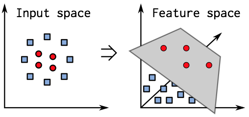
It could be describe as the transformation of raw data to produce a model input which will have better performance. The features are the new variables created in the process. It is often described as based on domain knowledge and more of an art than of a science. Therefore, it requires a great attention and a more “manual” process than the rest of data science projects.
Feature engineering tends to be heavier when raw data are far from the expected input format of our learning models (images or text for instance). It can be noticed that some feature engineering was already performed on our data, since banknotes were registered as images taken from a digital camera, and we only received 5 features for each image.
Correlated variables
Simple linear and polynomial regression
We noticed some strong dependencies between variables thanks to the scatter plot. Those can deter the performance and robustness of several machine learning models. Skewness and kurtosis seem to be somehow related. A regression line can be fitted with the skewness as explanatory variable:
a, b = stats.linregress(data0["skew"],data0["kurtosis"])[:2]
plt.plot(data0["skew"],data0["kurtosis"],'g+')
plt.plot(np.arange(-2.5,2.5,0.05) ,b+a*np.arange(-2.5,2.5,0.05),'r')
plt.title('Simple linear regression')
plt.xlabel('Skewness')
plt.ylabel('Kurtosis')
plt.show()
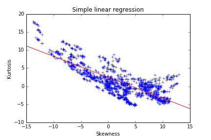
The following result highlights a lack in the model. The slope and intercept seem to be biased by a dense cluster of points with the skewness between 1 and 2. The points with a low skewness are under-represented in the model and do not follow the trend of the regression line. A robust regression technique could correct this bias, but a polynomial regression is the most straight-forward method to capture a higher part of the variance here. The second-degree polynomial model can be written as:
y_hat = a*np.square(x) + b*x + cand its coefficients can be determined through the minimization of least-square error in numpy:
a, b, c = np.polyfit(data0["skew"],data0["kurtosis"],deg=2)
plt.plot(data0["skew"],data0["kurtosis"],'+')
plt.plot(np.arange(-15,15,.5),a*np.arange(-15,15,.5) * np.arange(-15,15,.5)+b*np.arange(-15,15,.5)+c,'r')
plt.title('2nd degree polynomial regression')
plt.xlabel('Skewness')
plt.ylabel('Kurtosis')
A polynomial regression yields a much better output with balanced residuals. The p-value for all coefficients is below the 1% confidence criterion. One strong drawback can however be noticed: the polynomial model predicts an increase in the kurtosis for skewness superior to 2, but there is no evidence for this statement in our data, so the model could lead to stronger errors.
The regression does not capture all the variance (and does not explain all underlying phenomena) of the Kurtosis, so a transformed variable has to be kept, which should be independent from the skewness. The most obvious value is the residual of the polynomial regression we performed.
We can can represent this residual versus the explanatory variable to be assured that:
- The residuals are centered around 0
- The variance of the residuals is approximately constant with the skewness
- There are still patterns in the Kurtosis: the residuals are not just noise
p0 = plt.scatter(d0['skew'],c+b*d0["skew"] +a*d0["skew"]* d0["skew"]-d0["kurtosis"],c='b',marker='+',label="0")
p0 = plt.scatter(d1['skew'],c+b*d1["skew"] +a*d1["skew"]* d1["skew"]-d1["kurtosis"],c='r',marker='+',label="1")
plt.title('Explanatory variable vs Regression residuals')
plt.xlabel('Skewness')
plt.ylabel('Residuals')
plt.legend(["0","1"])
plt.show()
The data is now much more uncorrelated, so the feature of interest is the residual of the regression which will replace the kurtosis in the data.
Class-dependent regression
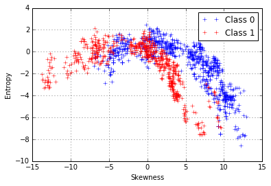
We can try and repeat the same process for the entropy and skewness, which also seem to be related to each other.
p0 = plt.scatter(d0['skew'],c+b*d0["skew"] +a*d0["skew"]* d0["skew"]-d0["kurtosis"],c='b',marker='+',label="0")
p0 = plt.scatter(d1['skew'],c+b*d1["skew"] +a*d1["skew"]* d1["skew"]-d1["kurtosis"],c='r',marker='+',label="1")
plt.title('Explanatory variable vs Regression residuals')
plt.xlabel('Skewness')
plt.ylabel('Residuals')
plt.legend(["0","1"])
plt.show()
plt.plot(d0["skew"],d0["entropy"],'+',label="Class 0")
plt.plot(d1["skew"],d1["entropy"],'r+',label="Class 1")
plt.xlabel("Skewness")
plt.ylabel("Entropy")
plt.grid()
plt.legend()
plt.show()
We can try can fit a 2nd-degree polynomial function:
ft = np.polyfit(data0["skew"],data0["entropy"],deg=2)
plt.plot(d0["skew"],d0["entropy"],'+',label="Class 0")
plt.plot(d1["skew"],d1["entropy"],'r+',label="Class 1")
plt.plot(np.arange(-15,14.5,.5),
         ft[0]*np.arange(-15,14.5,.5)*np.arange(-15,14.5,.5)+ft[1]*
         np.arange(-15,14.5,.5)+ft[2],'-',linewidth=2 ,
         label="Fitted polynom")
plt.xlabel("Skewness")
plt.ylabel("Entropy")
plt.grid()
plt.legend(loc="bottom center")
plt.show()
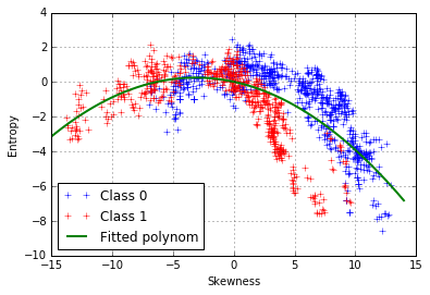
However, it seems that the model does not fit well our data and that the points are not equally distributed on both side of the curve. There is another pattern, which is class-dependent, so two polynomial curves should be fitted, one for each class:
f0 = np.polyfit(d0["skew"],d0["entropy"],deg=2)
x = np.arange(-15,14,.5)
f1 = np.polyfit(d1["skew"],d1["entropy"],deg=2)

plt.plot(x,f0[0]* x*x+f0[1]* x+f0[2],'-',label="Fitted 0")
plt.plot(d0["skew"],d0["entropy"],'+',alpha=.7,label="Class 0")

plt.plot(x,f1[0] * x*x+f1[1]* x+f1[2],'-',label="Fitted 1")
plt.plot(d1["skew"],d1["entropy"],'m+',alpha=.7,label="Class 1")

plt.title("Class dependent fit")
plt.xlabel("Skewness")
plt.ylabel("Entropy")
plt.grid()
plt.legend(loc='bottom center')
plt.savefig("class_depend.png")
plt.show()
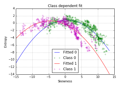
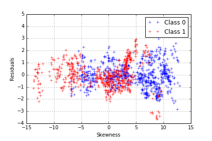
The model seems to capture more of the variance in our data, which we can confirm by plotting the residuals of the class-dependent regression.
plt.plot(d0["skew"],f0[0]* d0["skew"]* d0["skew"]+f0[1]* d0["skew"]+
        f0[2]-d0["entropy"],'b+',label="Class 0")
plt.plot(d1["skew"],f1[0]* d1["skew"]* d1["skew"]+f1[1]* d1["skew"]+
        f1[2]-d1["entropy"],'r+',label="Class 1")
plt.legend()
plt.grid()
plt.xlabel("Skewness")
plt.ylabel("Residuals")
plt.savefig("res_class_dep.png")
plt.show()
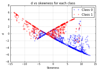
We have a proper working model, with just one problem: we used the class to predict the entropy whereas our classification objective is to proceed the other way around. Since we noticed that each class follows a different curve, a difference between the distance to the first model and the distance to the second model, which will be noted “d”, can be computed as:
d = np.abs(y - x.apply(f0)) - np.abs(y-x.apply(f1))A positive “d” value indicates that the entropy of the observation is closer to the model fitted on the class 1, this seems to be a rather relevant indicator to use to build our models. However, this variable seems correlated to the skewness. The latter could have become unnecessary for our prediction, so we choose to eliminate it from the features and take the risk of an information loss.
d = abs(data0["entropy"]-f0[0]* data0["skew"]* data0["skew"]-f0[1]* data0["skew"]-f0[2])-\
    abs(data0["entropy"]-f1[0]* data0["skew"]* data0["skew"]-f1[1]* data0["skew"]-f1[2])

d0["d"] = d[data0["class"]==0]
d1["d"] = d[data0["class"]==1]

plt.grid()
plt.plot(d0["skew"],d0["d"],'b+',label="Class 0")
plt.plot(d1["skew"],d1["d"],'r+',label="Class 1")
plt.legend()
plt.title("d vs skewness for each class")
plt.xlabel("Skewness")
plt.ylabel("d")
plt.show()
Variable scaling
Common scaling techniques
Very different spreads could be noticed among variables during the exploratory part. This can lead to a bias in the distance between two points. A possible solution to this is scaling or standardization.
-
Variance scaling of a variable is the division of each value by the variable standard deviation. The output is a variable with variance 1.
-
Min-Max standardization of a variable is the division of each value by the difference between the maximum and minimum values. The outcome values are all contained in the interval [0,1].
x_stand = x/(x.max()-x.min())Other standardization operations exist, but those are the most common because of the properties highlighted.
Advantages and risks
Scaling variables may avoid the distance between data points to be over-influenced by high-variance variables, because the ability to classify the data points from a variable is usually not proportional to the variable variance.
Furthermore, all people with notions in physics and calculus would find it awkward to compute a distance from heterogeneous variables (which would have different units and meaning).
However, scaling might increase the weight of variables carrying mostly or only noise, to which the model would fit, increasing the error on new data.
For this case, the second risk seems very low: all variables seem to carry information, which we could observe because of the low number of variables.
Feature engineering pipeline
a, b, c = np.polyfit(data0["skew"],data0["kurtosis"],deg=2)

data1 = data0.copy() # copying the data

data1.columns = ['vari', 'skew', 'k_resid', 'entropy', 'class']
data1["k_resid"] = data0["kurtosis"] - np.square(a*(data0["skew"]) + b*data0["skew"] + c)

data1.columns  = ['vari', 'skew', 'k_resid', 'd', 'class'] # computing the feature from the entropy regression

f0 = np.polyfit(d0["skew"],d0["entropy"],deg=2)
f1 = np.polyfit(d1["skew"],d1["entropy"],deg=2)

data1["d"] = abs(data0["entropy"]-f0[0]* data0["skew"]* data0["skew"]-f0[1]* data0["skew"]-f0[2])-\
    abs(data0["entropy"]-f1[0]* data0["skew"]* data0["skew"]-f1[1]* data0["skew"]-f1[2])

data1 = data1.drop("skew",1) # removing skew

data1.iloc[:,:4] = data1.iloc[:,:4]/np.sqrt(np.var(data1.iloc[:,:4])) # data normalization
data1 can now be used in the next step which will consist in the
implementation of a basic machine learning algorithm. This is the key
part in an analysis-oriented data science project, and I hope to see you there.
Mathieu Besançon
Researcher in mathematical optimization
Mathematical optimization, scientific programming and related.