
DifferentialEquations.jl - part 2: decision from the model
In the last article, we explored different modeling options for a three-component systems which could represent the dynamics of a chemical reaction or a disease propagation in a population. Building on top of this model, we will formulate a desirable outcome and find a decision which maximizes this outcome.
In addition to the packages imported in the last post, we will also use BlackBoxOptim.jl:
import DifferentialEquations
const DiffEq = DifferentialEquations
import Plots
import Optim
The model
The same chemical system with three components, A, B and R will be used: $$A + B → 2B$$ $$B → R$$
The reactor where the reaction occurs must remain active for one minute. Let’s imagine that $B$ is our valuable component while $R$ is a waste. We want to maximize the quantity of $B$ present within the system after one minute, that’s the objective function. For that purpose, we can choose to add a certain quantity of new $A$ within the reactor at any point. $$t_{inject} ∈ [0,t_{final}]$$.
Implementing the injection
There is one major feature of DifferentialEquations.jl we haven’t explored yet: the event handling system. This allows for the system state to change at a particular point in time, depending on conditions on the time, state, etc…
# defining the problem
const α = 0.8
const β = 3.0
diffeq = function(du, u, p, t)
    du[1] = - α * u[1] * u[2]
    du[2] = α * u[1] * u[2] - β * u[2]
    du[3] = β * u[2]
end
u0 = [49.0;1.0;0.0]
tspan = (0.0, 1.0)
prob = DiffEq.ODEProblem(diffeq, u0, tspan)

const A_inj = 30
inject_new = function(t0)
    condition(u, t, integrator) = t0 - t
    affect! = function(integrator)
        integrator.u[1] = integrator.u[1] + A_inj
    end
    callback = DiffEq.ContinuousCallback(condition, affect!)
    sol = DiffEq.solve(prob, callback=callback)
    sol
end

# trying it out with an injection at t=0.4
sol = inject_new(0.4)
Plots.plot(sol)
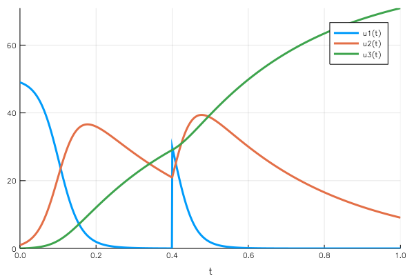
The ContinuousCallback construct is the central element here, it takes as
information:
- When to trigger the event, implemented as the
conditionfunction. It triggers when this function reaches 0, which is here the case when $t = t_0$. - What to do with the state at that moment. The state is encapsulated within the integrator variable. In our case, we add 30 units to the concentration in A.
As we can see on the plot, a discontinuity appears on the concentration in A at the injection time, the concentration in B restarts increasing.
Finding the optimal injection time: visual approach
From the previously built function, we can get the whole solution with a given injection time, and from that the final state of the system.
tinj_span = 0.05:0.005:0.95
final_b = [inject_new(tinj).u[end][2] for tinj in tinj_span]
Plots.plot(tinj_span, final_b)
Using a plain for comprehension, we fetch the solution of the simulation for the callback built with each $t_{inject}$.
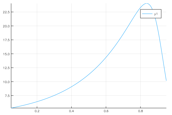
Injecting $A$ too soon lets too much time for the created $B$ to turn into $R$, but injecting it too late does not let enough time for $B$ to be produced from the injected $A$. The optimum seems to be around ≈ 0.82,
Finding the optimum using Optim.jl
The package requires an objective function which takes a vector as input. In our case, the decision is modeled as a single variable (the injection time), it’s crucial to make the objective use a vector nonetheless, otherwise calling the solver will just explode with cryptic errors.
compute_finalb = tinj -> -1 * inject_new(tinj[1]).u[end][2]
Optim.optimize(compute_finalb, 0.1, 0.9)
We get a detailed result of the optimization including the method and iterations:
* Algorithm: Brent's Method
* Search Interval: [0.100000, 0.900000]
* Minimizer: 8.355578e-01
* Minimum: -2.403937e+01
* Iterations: 13
* Convergence: max(|x - x_upper|, |x - x_lower|) <= 2*(1.5e-08*|x|+2.2e-16): true
* Objective Function Calls: 14
The function inject_new we defined above returns the complete solution
of the simulation, we get the state matrix u, from which we extract the
final state u[end], and then the second component, the concentration in
B: u[end][2]. The optimization algorithm minimizes the objective, while we want
to maximize the final concentration of B, hence the -1 multiplier used for
compute_finalb.
We can use the Optim.jl package because our function is twice differentiable, the best improvement direction is easy to compute.
Extending the model
The decision over one variable was pretty straightforward. We are going to extend it by changing how the $A$ component is added at $t_{inject}$. Instead of being completely dissolved, a part of the component will keep being poured in after $t_{inject}$. So the decision will be composed of two variables:
- The time of the beginning of the injection
- The part of $A$ to inject directly and the part to inject in a continuous fashion. We will note the fraction injected directly $\delta$.
Given a fixed available quantity $A₀$ and a fraction to inject directly $\delta$, the concentration in A is increased of $\delta \cdot A₀$ at time $t_{inject}$, after which the rate of change of the concentration in A is increased by a constant amount, until the total amount of A injected (directly and over time) is equal to the planned quantity.
We need a new variable in the state of the system, $u_4(t)$, which stands for the input flow of A being active or not.
- $u(t) = 0$ if $t < t_{inject}$
- $u(t) = 0$ if the total flow of A which has been injected is equal to the planned quantity
- $u(t) = \dot{A}\ $ otherwise, with $\dot{A}\ $ the rate at which A is being poured.
New Julia equations
We already built the key components in the previous sections. This time we need two events:
- A is directly injected at $t_{inject}$, and then starts being poured at constant rate
- A stops being poured when the total quantity has been used
const inj_quantity = 30.0;
const inj_rate = 40.0;

diffeq_extended = function(du, u, p, t)
    du[1] = - α * u[1] * u[2] + u[4]
    du[2] = α * u[1] * u[2] - β * u[2]
    du[3] = β * u[2]
    du[4] = 0.0
end

u0 = [49.0;1.0;0.0;0.0]
tspan = (0.0, 1.0)
prob = DiffEq.ODEProblem(diffeq_extended, u0, tspan)
We wrap the solution building process into a function taking the starting time and the fraction being directly injected as parameters:
inject_progressive = function(t0, direct_frac)
condition_start(u, t, integrator) = t0 - t
affect_start! = function(integrator)
integrator.u[1] = integrator.u[1] + inj_quantity * direct_frac
integrator.u[4] = inj_rate
end
callback_start = DiffEq.ContinuousCallback(
condition_start, affect_start!, save_positions=(true, true)
)
condition_end(u, t, integrator) = (t - t0) * inj_rate - inj_quantity * (1 - direct_frac)
affect_end! = function(integrator)
integrator.u[4] = 0.0
end
callback_end = DiffEq.ContinuousCallback(condition_end, affect_end!, save_positions=(true, true))
sol = DiffEq.solve(prob, callback=DiffEq.CallbackSet(callback_start, callback_end), dtmax=0.005)
end
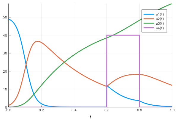
Plots.plot(inject_progressive(0.6,0.6))We can notice callback_start being identical to the model we previously built,
while condition_end corresponds to the time when the total injected
quantity reaches inj_quantity. The first events activates $u_4$ and sets it
to the nominal flow, while the second callback resets it to 0.
Optim.jl can be re-used to determine the optimal decision:
objective = function(x)
    sol = inject_progressive(x[1], x[2])
    -sol.u[end][2]
end
# wrapped objective function and starting point
x0 = 0.5*ones(2)
wrapped_obj = Optim.OnceDifferentiable(objective, x0)
# call optimize with box algorithm
Optim.optimize(wrapped_obj, x0, [0.1,0.0], [1.0,1.0], Optim.Fminbox())
The result details are:
* Algorithm: Fminbox with Conjugate Gradient
* Starting Point: [0.5,0.5]
* Minimizer: [0.8355419400368459,0.9999654432422779]
* Minimum: -2.404040e+01
* Iterations: 4
* Convergence: true
  * |x - x'| ≤ 1.0e-32: false
    |x - x'| = 3.43e-04
  * |f(x) - f(x')| ≤ 1.0e-32 |f(x)|: true
    |f(x) - f(x')| = -6.85e-11 |f(x)|
  * |g(x)| ≤ 1.0e-08: false
    |g(x)| = 9.05e-08
  * Stopped by an increasing objective: true
  * Reached Maximum Number of Iterations: false
* Objective Calls: 125
* Gradient Calls: 79
We wrap our function in a Optim.OnceDifferentiable to provide Optim with the
information that the function is differentiable, even though we don’t provide a
gradient, it can be computed by automatic differentiation or finite differences.
The optimal solution corresponds to a complete direct injection ($\delta \approx 1$) with $t_{inject}^{opt}$ identical to the previous model. This means pouring the A component in a continuous fashion does not allow to produce more $B$ at the end of the minute.
Conclusion
We could still built on top of this model to keep refining it, taking more phenomena into account (what if the reactions produce heat and are sensitive to temperature?). The structures describing models built with DifferentialEquations.jl are transparent and easy to use for further manipulations.
One point on which I place expectations is some additional interoperability between DifferentialEquations.jl and JuMP, a Julia meta-package for optimization. Some great work was already performed to combine the two systems, one use case that has been described is the parameter identification problem (given the evolution of concentration in the system, identify the α and β parameters).
But given that the function I built from a parameter was a black box (without an explicit formula, not a gradient), I had to use BlackBoxOptim, which is amazingly straightforward, but feels a bit overkill for smooth functions as presented here. Maybe there is a different way to build the objective function, using parametrized functions for instance, which could make it transparent to optimization solvers.
If somebody has info on that last point or feedback, additional info you’d like to share regarding this post, hit me on Twitter. Thanks for reading!
Edits and improvements
2018-01-31:
I updated this post to adapt to the new DifferentialEquations.jl
interface. I also used Optim.jl for the two cases without BlackBoxOptim.jl,
which is very nice but not necessary for differentiable functions.
Special thanks to Patrick for his quick response
and help with Optim.jl.
2017-12-20:
Of course, BlackBoxOptim.jl was not the most appropriate algorithm as
predicted. Patrick and Chris
gave me some hints in this thread
and I gave Optim.jl a try.
This package has a range of algorithms to choose from depending on the structure of the function and the knowledge of its gradient and Hessian. The goal is continuous optimization, (as opposed to BlackBoxOptim.jl which supports more exotic search spaces).
Finding the optimum $t_{inject}$ of the first problem is pretty simple:
import Optim
Optim.optimize(compute_finalb, 0.1, 0.9)
This yields the following information:
Results of Optimization Algorithm
 * Algorithm: Brent's Method
 * Search Interval: [0.100000, 0.900000]
 * Minimizer: 8.355891e-01
 * Minimum: -2.403824e+01
 * Iterations: 13
 * Convergence: max(|x - x_upper|, |x - x_lower|) <= 2*(1.5e-08*|x|+2.2e-16): true
 * Objective Function Calls: 14
14 calls to the objective function, pretty neat compared to the hundreds of
BlackBoxOptim. We also confirm the optimum of 0.8355891. Not yet sure we could
use Optim.jl for the second case (boxed multivariate optimization without explicit gradient).
Mathieu Besançon
Researcher in mathematical optimization
Mathematical optimization, scientific programming and related.